Block3: Erregungsleitung
Myelogenese ZNS, PNS; Dekrement; Kreisströmchen; Saltatorische Ausbreitung;Frequenz/Amplituden-Modulation, Regeneration; Querschnittslähmung, Therapie-Aussichten
Fragen:
- Worin unterscheidet sich Reizleitung von Erregungsleitung und welche Strecken können/müssen Erregungen zurücklegen?
- Was versteht man unter Erregungsausbreitung mit Dekrement und welche Vorteile haben Aktionspotenziale AP?
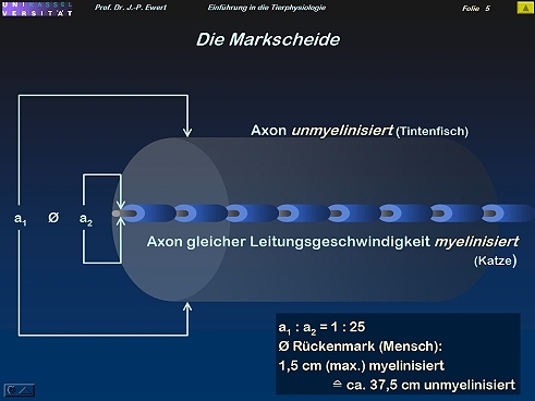
- Welche Vorteile hat die segmentale Ummantelung des Axons durch Markscheiden bestehend aus Myelinschichten (Myelinisierung)?
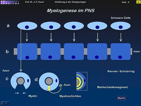
- Wie entstehen Markscheiden im peripheren Nervensystem?
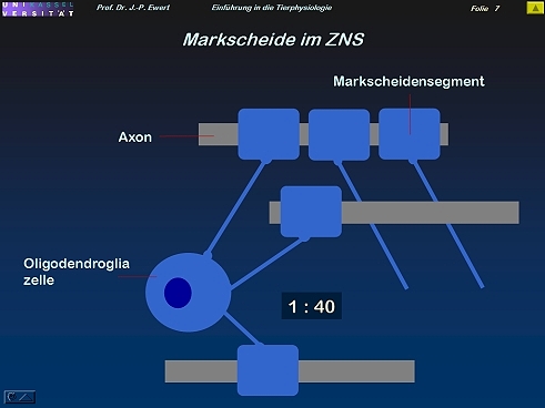
- Wie entstehen Markscheiden im Zentralnervensystem?
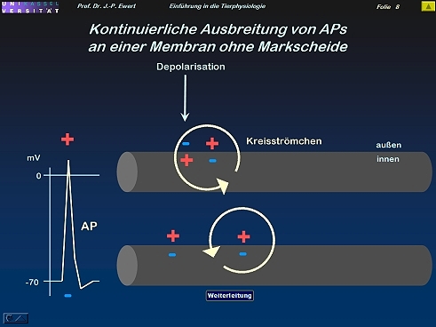
- Wie verschieben sich Ladungen durch Kreisströmchen bei der AP-Ausbreitung?
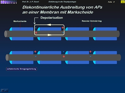
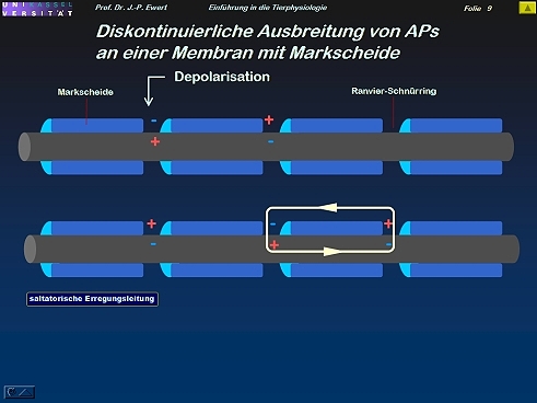
- Welche Vorteile hat die saltatorische AP-Ausbreitung längs des myelinisierten Axons?
- Wie werden Signale kodiert und an einer exzitatorischen Synapse dekodiert?
- Wie werden Signale an einer inhibitorischen Synapse dekodiert?
- Auf welchen Prinzipien beruht AP-Frequenzkodierung?
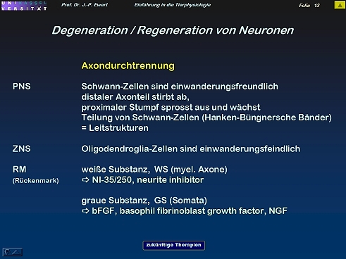
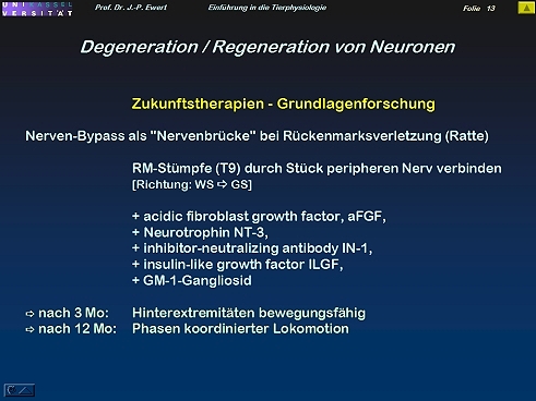
- Können Neurone nach Verletzung regenerieren bzw. sind Neurone ersetzbar?
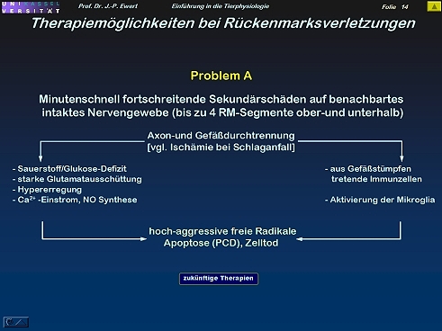
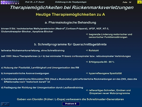
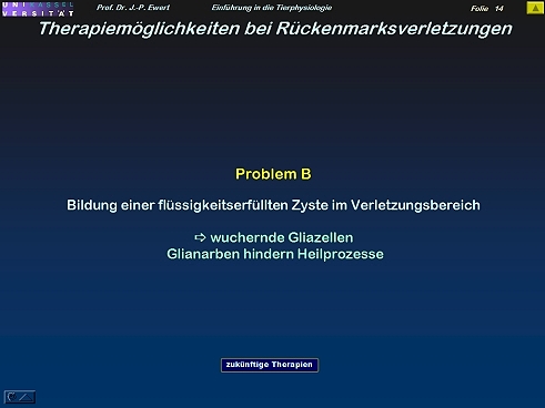
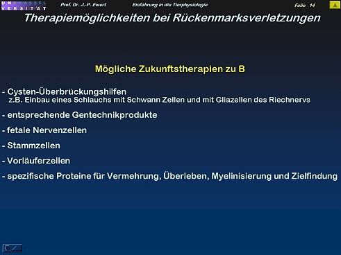
- Welche schnellen Sekundärschäden setzen nach einer Rückenmarksverletzung ein und welche Therapiemöglichkeiten gibt es?
Folien:
Ein Axon eines Neurons aus dem Gehirn eines Dinosauriers (Barosaurus), das in der Schwanzspitze endigte, konnte ca. 27 m lang sein
1

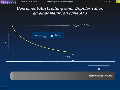
Was versteht man unter Erregungsausbreitung mit Dekrement und welche Vorteile haben Aktionspotenziale?
2
Welche Vorteile hat die Myelinisierung?
3
Wie entstehen Markscheiden im peripheren Nervensystem?
4
Wie entstehen Markscheiden im Zentralnervensystem?
5
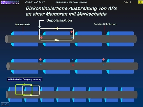
Wie verschieben sich Ladungen durch Kreisströmchen längs des Axon bei der AP-Ausbreitung?
6
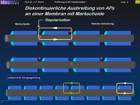
Welche Vorteile hat die saltatorische AP-Ausbreitung längs des Myelinisierten Axons?
7
Unten: Geschwindigkeit der AP-Ausbreitung am unmyelinisierten (grün) und myelinisierten Axon (weiß)
8
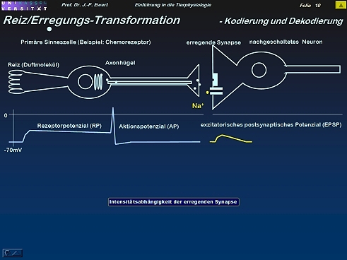
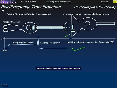
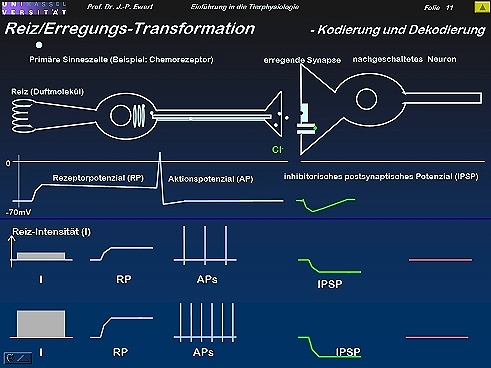
Wie werden Signale kodiert und an einer exzitatorischen Synapse dekodiert?
9
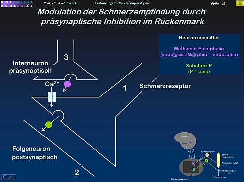
Wie werden Signale an einer inhibitorischen Synapse dekodiert?
10
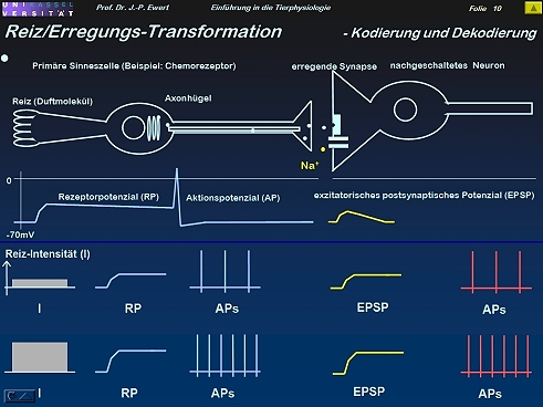
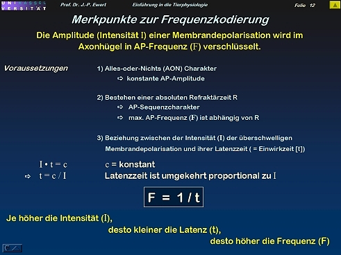
Auf welchen Prinzipien beruht AP-Frequenzkodierung?
11
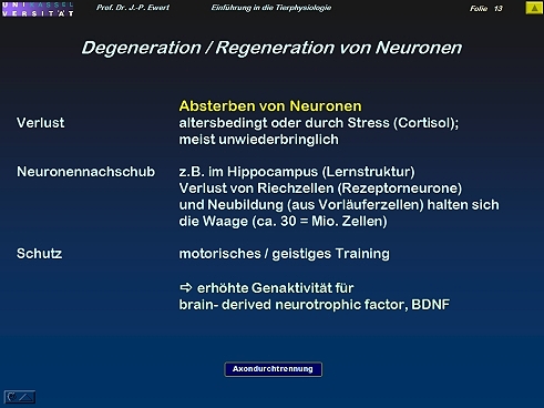
Können Neurone nach Verletzung regenerieren bzw. sind Neurone ersetzbar?
12
.
Welche schnellen Sekundärschäden setzen nach Rückenmarksverletzungen ein und welche Therapiemöglichkeiten gibt es ?
13
_______________________________________________________
Block4: Synaptische Übertragungen
Schnelle/Langsame(2nd-Messenger)Synapsen; Vesikel-Prozesse; Gedächtnis, Signaltransduktionen, cAMP, IP3; Rechenoperationen; NO-gesteuerte Prozesse
Fragen:
- Welche Einzelschritte lassen sich an einer "schnellen Synapse" unterscheiden?
- Nach welchem Prinzip öffnet Acetylcholin einen Na+ Ionenkanal?
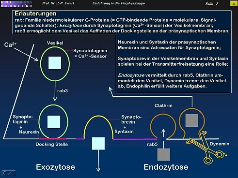
- Wo und wie werden synaptische Vesikel gebildet?
- Welche Vesikelmembran-Interaktionen finden bei Exozytose und Endozytose statt?
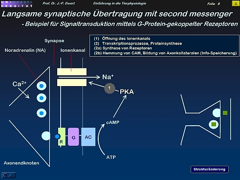
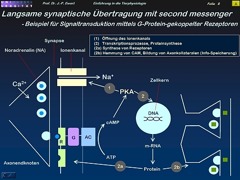
- Über welche Signal-Transduktionen induziert ein Neurotransmitter an "langsamen Synapsen" strukturelle Veränderungen im Zusammenhang mit langfristiger Informationsspeicherung?
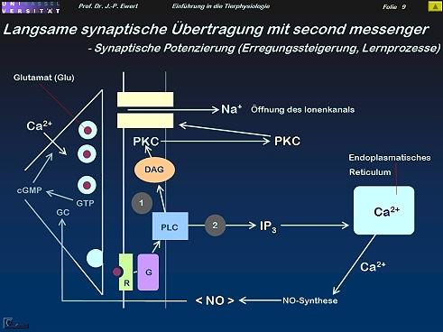
- Welche Signalkette führt rückwirkend zur Steigerung (Potenzierung) der synaptischen Übertragung?
- Synapsen gleichen elektronischen Modulen: Wie werden neuronale Aktivitäten summiert?
- Synapsen gleichen elektronischen Modulen: Wie werden neuronale Aktivitäten subtrahiert?
- Synapsen gleichen elektronischen Modulen: Wie wird multipliziert, z.B. Faktor <1 ?Schmerzausschaltung: Wie lässt sich synaptische Übertragung beeinflussen?
Folien:
Welche Einzelschritte lassen sich an einer "schnellen Synapse" unterscheiden?
1
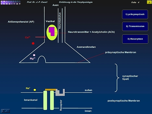
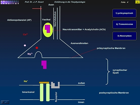

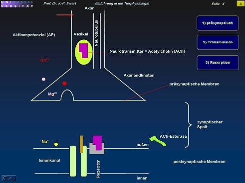
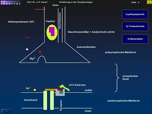
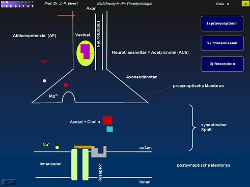
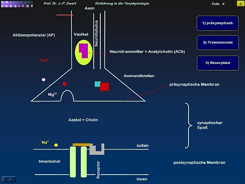
Nach welchem Prinzip öffnet Acetylcholin einen Na+ Ionenkanal?
2
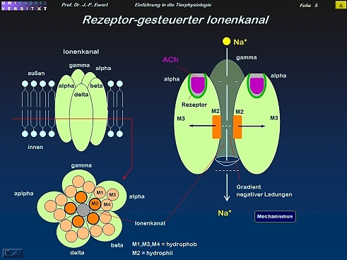
(Abstrahiert und kombiniert nach Zimmermann 1996)
Wo und wie werden synaptische Vesikel gebildet?
3
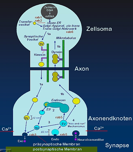
 (Modifiziert nach Wucherpfennig 2002)
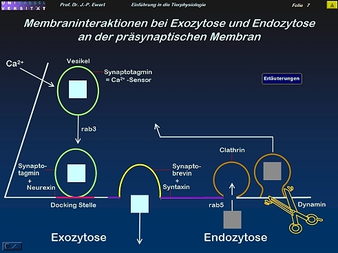
Welche Vesikelmembran-Interaktionen finden bei synaptischer Exozytose und Endozytose statt?
4
 .
.
(Abstrahiert und kombiniert nach Zimmermann 1996)
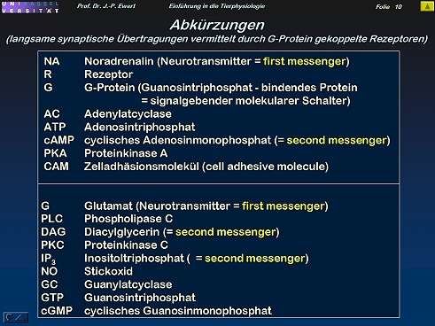
Über welche Signal-Transduktionen induziert ein Neurotransmitter an "langsamen Synapsen" strukturelle Veränderungen im Zusammenhang mit langfristiger Informationsspeicherung?
5
Welche Signalkette führt rückwirkend zur Steigerung (Potenzierung) der synaptischen Übertragung?
6
7
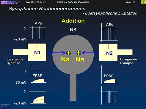
Synapsen gleichen elektronischen Modulen: Wie werden neuronale Aktivitäten summiert?
8
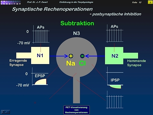
Synapsen gleichen elektronischen Modulen: Wie werden neuronale Aktivitäten subtrahiert?
9
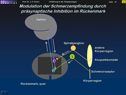
Synapsen gleichen elektronischen Modulen: Wie werden neuronale Aktivitäten multipliziert (z.B. Faktor <1)?
Beispiel: Schmerzausschaltung mittels Akupunktur durch präsynaptische Inhibition im Rückenmark
10
.